representing a shear/skew with only rotation and scaling

posted 2025-06-26T08:07:00Z

clickbait title: “rederiving an extremely elegant equation from a classic 1990 computer graphics book”

note: this post uses MathML for formatting the math. it looks a little weird on chromium-based browsers, but firefox should look good

I’m in resonite–as I am–hanging out with some critters in a world–as one does. sparsely out of the corner of my eyes and ears, I oversee and overhear someone else in the session messing about with a cube, cursing at how the math they’re doing isn’t working out. of course, I hear the word “math” and perk up immediately, going over to observe their happenings. what was their plight? what accursed math must they be doing to provoke this reaction? fumbling with quaternions? higher-dimensional happenings and mappings?

turns out, they just wanted to shear a cube. that’s right–this funny little transformation:

and it was ending up being harder than they thought. I was then ~~conscripted~~ nerd sniped into figuring this out as well, which took up approximately four full days of time thinking about this problem and gaining knowledge of a neat little linear algebra thing in the process, hence why I am writing this post about it.

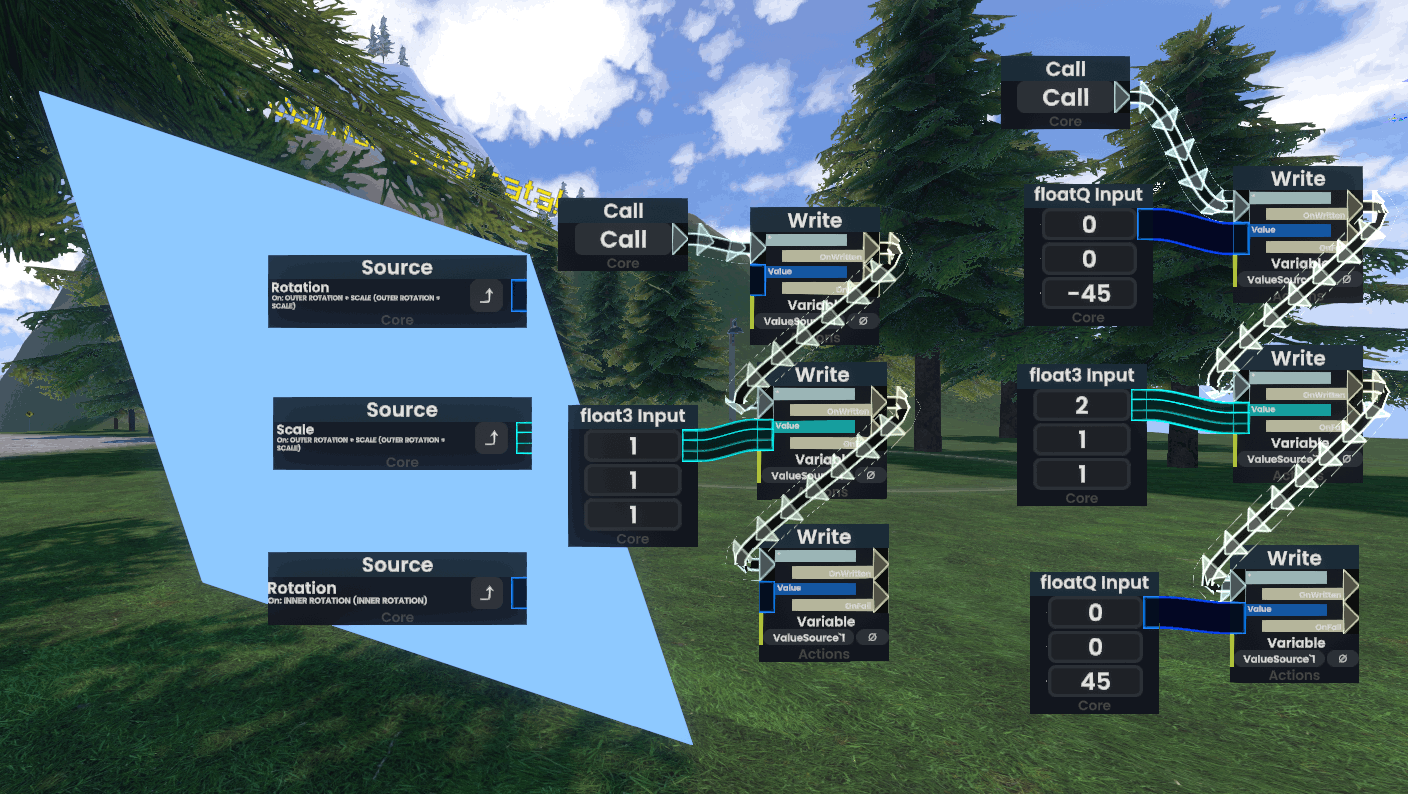
for reference, in resonite, components for meshes, rendering, all the like are attached to things called “slots”. these slots make up a hierarchy in the world, and each slot can have a transformation applied to it. however, you only have access to translation, rotation, and scaling on any individual slot. as such, if you want to express complex, arbitrary transformations on components, you have to compose the transformations on these individual slots. you do not have access to arbitrary transformations directly–all transformations have to eventually be represented in this hierarchy of slots alone.

as an example, if I want to stretch out a cube along one of its axis-aligned diagonal, I have to:

rotate the cube by 45 degrees (inner slot)
scale the cube in the desired direction (outer slot)
rotate the cube back 45 degrees (outer slot)

A visual demonstration of the above steps

now you might be able to see where the problem lies.

my initial attempt

I came into this armed with a heap of trigonometry knowledge, so I took a crack at trying to solve this myself. I & the other critter came up with the process of:

rotate the object 45 degrees towards the skew direction
scale the object in the direction of skew
undo the rotation with some trig at the end
undo the deformation that results from the scaling in step 2

and I was the one to figure out the number crunching and equation solving for it.

this idea actually worked!… kinda. there were two issues with it:

it required four transformations, or at minimum 3 slots (the scale and undo-rotation in step 2 and 3 can be done in one slot). I was under the impression that this has to be possible in only 3 transformations, or two slots
it only worked for angles up to 45 degrees. while the object can stretch infinitely long in step 2, that stretch has to be compensated for in step 4 to preserve the side lengths on axes that shouldn’t be affected by the skew. this would cause the transformation to get closer and closer to 45 degrees… but never truly reach it.

here’s the three pages of work I scrawled while figuring out this method:

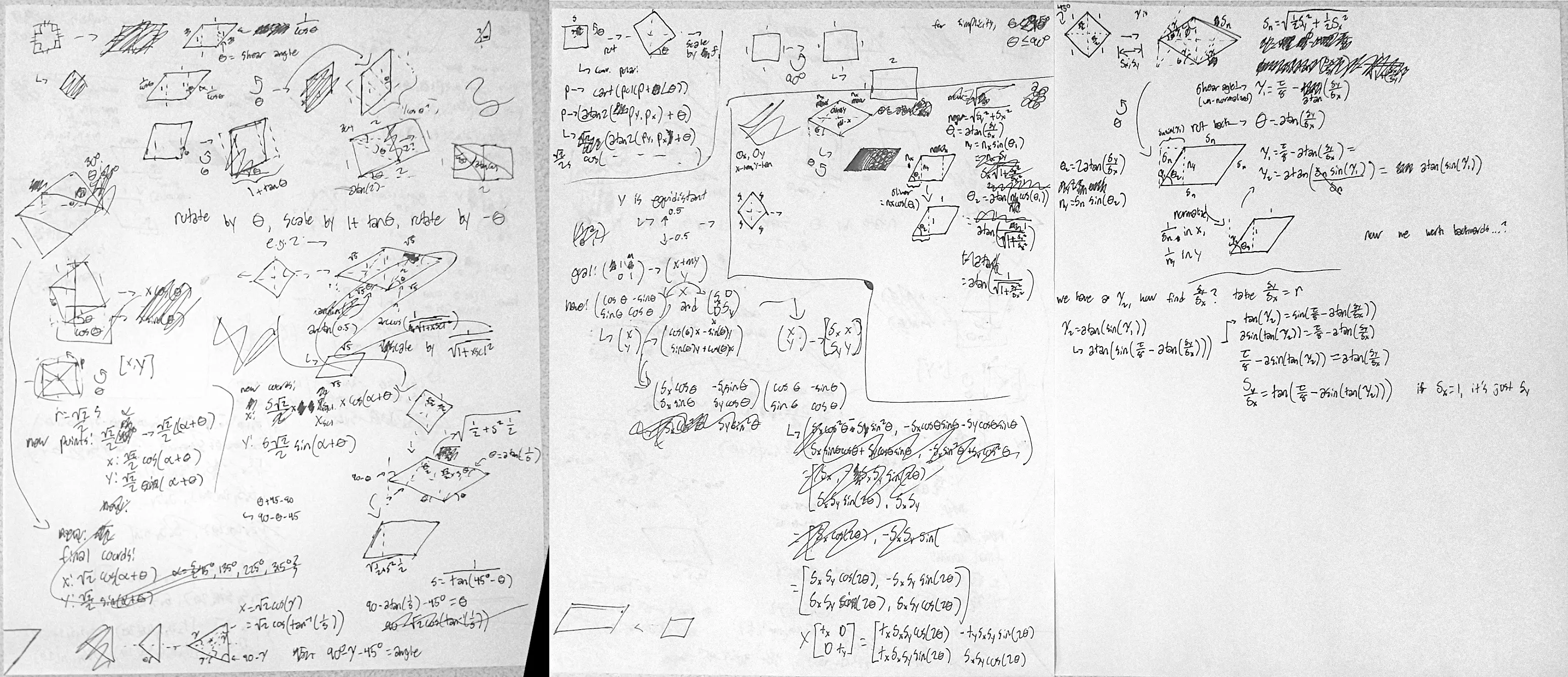
Three pages of trigonometry. there’s a lot of functions, rhombuses, and triangles present.

you can notice how I had the idea of using non-45 degree angles to prevent the limit that 45 degrees caused, but analyzing that with only trigonometry got way too unwieldy for me to pursue. as such, I decided that it was time to start thinking more analytically

problem statement

the basic premise of a shear/skew is this: we want to scale one axis based on how far along another axis we are. this causes points close to the zero line of the shear axis to move only a little bit, while points far away from the shear axis to move a lot. this can be seen visually in the image back at the top of this post.

to progress in this endeavor, however, it would help a lot to represent this analytically. we leave the land of geometry and trig for the land of matrices. unfortunately, I will not be explaining everything there is to do with matrices for this post–it would be too much and sprawl the post out too much–but there are excellent resources online to get started with them. to reduce clutter further, I will only be looking at the 2d case throughout most of this post–the 3d case follows directly from the 2d concepts.

to begin, a shearing matrix looks like this:

\begin{bmatrix}1&a\\ 0&1\end{bmatrix}

this accomplishes our goal of scaling one axis as we move along the other axis:

\begin{bmatrix}1&a\\ 0&1\end{bmatrix}\begin{bmatrix}x\\ y\end{bmatrix}=\begin{bmatrix}x+ay\\ y\end{bmatrix}

now, we want to represent this matrix with rotations and scaling only. I’ll save the complications and just state that translation is not needed throughout this entire thing. as a refresher, a rotation matrix looks like this:

\begin{bmatrix}\cos\theta&-\sin\theta\\ \sin\theta&\cos\theta\end{bmatrix}\begin{bmatrix}x\\ y\end{bmatrix}=\begin{bmatrix}x\cos\theta-y\sin\theta\\ x\sin\theta+y\cos\theta\end{bmatrix}

and a scale matrix looks like this:

\begin{bmatrix}S_{x}&0\\ 0&S_{y}\end{bmatrix}\begin{bmatrix}x\\ y\end{bmatrix}=\begin{bmatrix}xS_{x}\\ yS_{y}\end{bmatrix}

and to “compose” transformations, we just multiply the matrices together.

you can glance at these three matrices and quickly realize that this isn’t quite as trivial as it may seem. figuring out some special rotation and scale constants to cancel everything out to 1 along the diagonal, 0 in the bottom left, and a nonzero term in the top right is not something that can just be done in a human brain.

usually, when pursuing such a question, it’s best to first see if anyone else thought of this problem as well. time to start researching.

research

there’s not much existing information online about this specific conundrum. turns out, in most places where this might be an issue (such as Unity), you have access to arbitrary shader code, which means arbitrary transformations either way. it makes this kind of thing extremely niche and only really relevant in places where you’re hard-constrained to these basic three transformations–which describes my situation exactly.

nonetheless, I did find a few hints at a direction to look in, thanks to stackoverflow:

both of these questions pointed towards something I haven’t heard before–this thing called the “SVD”. following one of the links to this college homework assignment from 2003, question 3 gives more insight on this whole thing. while it displays a formula for a special case of a shear matrix, where the shear factor is $a-\frac{1}{a}$ , this is not a general form that made me happy. looking at the end of the question, a particular book is referenced: “Graphics Gems I”, page 485.

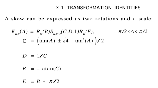
I went and acquired that book–in a totally legal manner, of course–and went to the page in question. on that page, the following equation is presented without comment:

The equation from Graphics Gems I, showcasing a lot of square roots and tangents

for some reason–and I didn’t realize this until writing this post–this section of the book (unsure about the whole book) shows all the matrices as their transposes than what you’d expect. their rotations are clockwise by default rather than counterclockwise by default–their skews not aligned with current conventions. they might be doing their matrix multiplication as right multiplications rather than the conventional left multiplication.

to translate this from the primitive formatting and backwards convention of the book, it states the following:

\begin{bmatrix}1&\tan a\\ 0&1\end{bmatrix}=R\left(\theta+\frac{\pi}{2}\right)\times\begin{bmatrix}\gamma% &0\\ 0&\frac{1}{\gamma}\end{bmatrix}\times R(\theta)

where

\begin{split}\gamma&=\frac{1}{2}\left(\tan(a)\pm\sqrt{\tan^{2}(a)+4}\right)\\ \theta&=-\arctan(\gamma)\end{split}

and $R$ is the rotation matrix as described above. if you want to change the direction of shear, you can simply swap the scale values and axis of rotation.

what a neat and elegant equation! I noticed that the $\tan a$ part was only necessary for knowing the angle of shear, and that I can just replace all the tangents in the equation with just a constant “shear factor”, simplifying it a bit.

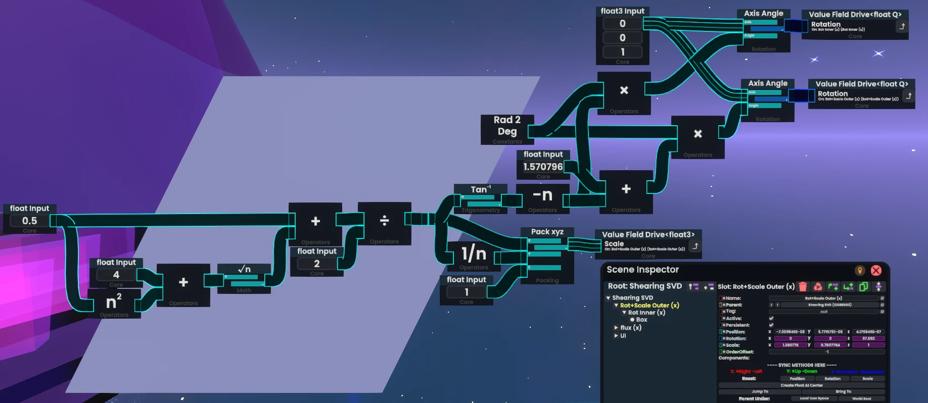
I went ahead and ported this to protoflux–resonite’s node-based programming language for this kind of thing–and it just, worked perfectly fine.

A cube being sheared in resonite

I was simultaneously excited that I found an implementation that worked, but also incredibly disappointed that I had no idea how it worked. how did they derive this? what thought process went in to this? of course, the book itself didn’t derive it at all. nothing in that entire section leds up to that formula, nor did they give any hint at how to derive it in the first place.

but if you remember, I was given a hint from stackoverflow & the homework: this silly little thing called the “singular value decomposition”

what the hell is a singular value

if you try and search what the singular value decomposition is online, chances are that you’ll get swamped with formalisms and definitions and have a very hard time. I was like this when looking at the wikipedia article about the subject, and I ended up obsessing over everything when it didn’t quite matter all the time.

I’ll assume you already know what a matrix is, the basic operations on them, and a few basic linear algebra terms related to them. I kinda already did that up above. it’ll also be helpful to know what an eigenvalue and eigenvector is. if you don’t, the wikipedia page for them is much more practically understandable than the SVD page.

before explaining the SVD, there’s a few quick facts you should internalize first:

the eigenvalues of $AA^{T}$ and $A^{T}A$ are the same.
the matrix products $AA^{T}$ and $A^{T}A$ are both symmetric matrices. this means that, for both of the matrices, their eigenvectors are orthogonal to each other, and thus can be used to construct an orthogonal matrix if you normalize them.

with these two facts in mind, here’s an hopefully intuitive understanding of what the SVD is, starting with an informal definition and building on it:

any matrix–and thus any linear transformation–can be represented as a multiplication of three special matrices:

$U$ : an orthogonal matrix
$\Sigma$ : a diagonal matrix
$V^{T}$ : a transpose of another orthogonal matrix, which means that it itself is also orthogonal

this is commonly notated like $A=U\Sigma V^{T}$ .

what does this mean for transformations? well, an orthogonal matrix is used to rotate things, and a diagonal matrix is used to scale things, so… any linear transformation can be represented as a rotation, followed by some scale, followed by another rotation. pretty neat, isn’t it?

to get specific about what these values are, the columns of the $U$ and $V$ matrices are made up of the normalized eigenvectors of the matrices $AA^{T}$ and $A^{T}A$ , respectively. these two sets of eigenvectors are called the left singular vectors and right singular vectors, respectively. the entries along the diagonal of $\Sigma$ are the square roots of the eigenvalues of $AA^{T}$ or $A^{T}A$ (since these two matrices have the same eigenvalues). they should align in the same columns as their corresponding eigenvectors in the other two matrices, and the most common convention for this is to put them in descending order along the diagonal.

why does this work?

recall what eigenvalues and eigenvectors are for a minute. if we can represent a matrix multiplied with a vector as a scalar multiplied with said vector, what would happen if we had a way to make a “base” of orthogonal eigenvectors, applying different scales to each eigenvector? we’d be able to represent that matrix transformation with only scaling. this is the essence of the SVD.

keeping in mind that the convention is to left-multiply the transformation matrix against the vector, this is the order of transformations:

when multiplying by $V^{T}$ , we rotate our coordinate space from our original basis–what we’d consider the “x” and “y” unit vectors geometrically–to the basis of the eigenvectors of $A^{T}A$ .
now that we’re in this coordinate space, we use the singular values to perform the transformation of A in the eigenspace of AT⁢A.
- I was confused as to why these singular values did this transformation, but I think I get it now. conventionally, when you square a matrix, the eigenvalues of that new matrix are the eigenvalues of the original matrix squared. this is not the case when you multiply a matrix by its transpose. however, when we’re in the basis of $A^{T}A$ , the eigenvalues of that product are doing that transformation in that basis, but squared. we have to account for this by square rooting the eigenvalues. this is just my line of reasoning that I am attempting to deduce from this and is in no way formal. if someone who knows about this more than me sees this and it’s completely wrong, let me know and I’ll edit this!
finally, after we do the transformation, we need to rotate back to our original basis. therefore, we multiply by $U$ composed of the left singular vectors.

deriving the shear case

that’s all well and good, but this was supposed to be about the shear transformation! oh dear. I’m 170 or so lines into this djot file and haven’t talked about the shear transformation yet. but no longer! because I will finally be showcasing the derivation of that one equation that I was so obsessed over. this will serve both as a more accessible reference for this equation, as well as a complete workout of computing the singular value decomposition, since there’s a severe lack of that on the internet. let’s go!

remember: the shear matrix looks like so:

A=\begin{bmatrix}1&a\\ 0&1\end{bmatrix}

the singular values

we first compute $AA^{T}$ and $A^{T}A$ :

\begin{split}AA^{T}&=\begin{bmatrix}1&a\\ 0&1\end{bmatrix}\begin{bmatrix}1&0\\ a&1\end{bmatrix}=\begin{bmatrix}1+a^{2}&a\\ a&1\end{bmatrix}\\ A^{T}A&=\begin{bmatrix}1&0\\ a&1\end{bmatrix}\begin{bmatrix}1&a\\ 0&1\end{bmatrix}=\begin{bmatrix}1&a\\ a&1+a^{2}\end{bmatrix}\end{split}

then we compute the eigenvalues of either of these two matrices. we don’t need to do both, since the eigenvalues for the two matrices are the same. going against sheldon axler for a moment here, we’ll get the characteristic polynomial:

\begin{split}\text{det}(A^{T}A)&=(1-\lambda)(1+a^{2}-\lambda)-a^{2}\\ &=1+a^{2}-\lambda-\lambda-a^{2}\lambda+\lambda^{2}-a^{2}\\ &=\lambda^{2}-(a^{2}+2)\lambda+1\end{split}

and solve for the eigenvalues, this time simply with the quadratic equation:

\begin{split}\lambda&=\frac{1}{2}\left(a^{2}+2\pm\sqrt{(-(a^{2}+2))^{2}-4}% \right)\\ &=\frac{1}{2}\left(a^{2}+2\pm\sqrt{a^{4}+4a^{2}+4-4}\right)\\ &=\frac{1}{2}\left(a^{2}+2\pm\sqrt{a^{4}+4a^{2}}\right)\end{split}

I’ll split the two eigenvalues up like so:

\begin{split}\lambda_{+}&=\frac{1}{2}\left(a^{2}+2+a\sqrt{a^{2}+4}\right)\\ \lambda_{-}&=\frac{1}{2}\left(a^{2}+2-a\sqrt{a^{2}+4}\right)\end{split}

where the square root always represents the positive square root.

note how $\lambda_{+}>\lambda_{-}$ for all values of $a$ .

to get the singular values from these, all we need to do is take the square root of these eigenvalues:

\begin{split}\sigma_{+}&=\sqrt{\lambda_{+}}\\ &=\sqrt{\frac{1}{2}\left(a^{2}+2+a\sqrt{a^{2}+4}\right)}\\ &=\frac{1}{2}\sqrt{2a^{2}+4+2a\sqrt{a^{2}+4}}\\ &=\frac{1}{2}\sqrt{\left(a+\sqrt{a^{2}+4}\right)^{2}}\\ &=\frac{1}{2}\left(a+\sqrt{a^{2}+4}\right)\end{split}

you can go through these same motions for $\lambda_{-}$ to find $\sigma_{-}$ :

\sigma_{-}=\frac{1}{2}\left(a-\sqrt{a^{2}+4}\right)

in the context of the SVD, these singular values are used to construct $\Sigma$ , the middle matrix, by placing them along the diagonals. the order of these values doesn’t really matter so long as the singular vectors corresponding to said eigenvalues are placed in the same columns of $U$ and $V$ . however, it’s a common convention to sort them in a descending order, making our middle matrix:

\Sigma=\begin{bmatrix}\sigma_{+}&0\\ 0&\sigma_{-}\end{bmatrix}

if you remember what the equation says, this seems ridiculous! both diagonal entries are stated in terms of only one number, not two like we have here. to remedy this, we can pull off some neat little algebra for a cool result:

\begin{split}\sigma_{-}&=\frac{a-\sqrt{a^{2}+4}}{2}\\ &=\frac{a-\sqrt{a^{2}+4}}{2}\left(\frac{a+\sqrt{a^{2}+4}}{a+\sqrt{a^{2}+4}}% \right)\\ &=\frac{a^{2}-a^{2}-4}{2\left(a+\sqrt{a^{2}+4}\right)}\\ &=-\frac{1}{\frac{1}{2}\left(a+\sqrt{a^{2}+4}\right)}\\ &=-\frac{1}{\sigma_{+}}\end{split}

which makes our $\Sigma$ :

\Sigma=\begin{bmatrix}\sigma_{+}&0\\ 0&-\frac{1}{\sigma_{+}}\end{bmatrix}

right singular vectors

now we need to find the eigenvectors of both of the matrices. even though the eigenvalues are the same, the eigenvectors are not. starting with the right singular vectors, we need to find the eigenvectors of $A^{T}A$ corresponding to our two eigenvalues:

$\lambda_{+}$ :

\begin{split}&\begin{bmatrix}1-\frac{1}{2}\left(a^{2}+2+a\sqrt{a^{2}+4}\right)% &a\\ a&1+a^{2}-\frac{1}{2}\left(a^{2}+2+a\sqrt{a^{2}+4}\right)\end{bmatrix}\begin{% bmatrix}v_{1}\\ v_{2}\end{bmatrix}=\bf{0}\\ &\Rightarrow\left\{\begin{array}[]{}-\frac{1}{2}\left(a^{2}+a\sqrt{a^{2}+4}% \right)v_{1}+av_{2}&=0\\ av_{1}-\frac{1}{2}\left(-a^{2}+\sqrt{a^{2}+4}\right)v_{2}&=0\end{array}\right.% \\ &\Rightarrow av_{2}=\frac{1}{2}\left(a^{2}+a\sqrt{a^{2}+4}\right)v_{1}\quad% \quad\text{(Using 1st equation)}\\ &\Rightarrow v_{2}=\frac{1}{2}\left(a+\sqrt{a^{2}+4}\right)v_{1}\\ &\Rightarrow\mathbf{v}_{+}=\begin{bmatrix}1\\ \frac{1}{2}\left(a+\sqrt{a^{2}+4}\right)\end{bmatrix}=\begin{bmatrix}1\\ \sigma_{+}\end{bmatrix}\end{split}

now we need to normalize this vector such that it can be used in an orthogonal matrix. if we look at the reciprocal of its length:

\frac{1}{\left\|\mathbf{v}_{+}\right\|}=\frac{1}{\sqrt{1^{2}+\sigma_{+}^{2}}}

hey, wait a minute… if we refer to wikipedia’s table of inverse trig identities, this is an identity!

\frac{1}{\sqrt{1+\sigma_{+}^{2}}}=\cos\left(\arctan\left(\sigma_{+}\right)\right)

this makes the normalized form of the eigenvector extremely simple:

\begin{split}\frac{\mathbf{v}_{+}}{\left\|\mathbf{v}_{+}\right\|}&=\begin{% bmatrix}\cos(\arctan(\sigma_{+}))\\ \cos(\arctan(\sigma_{+}))\sigma_{+}\end{bmatrix}\\ &=\begin{bmatrix}\cos(\arctan(\sigma_{+}))\\ \sin(\arctan(\sigma_{+}))\end{bmatrix}\end{split}

hooray! we have computed one of the right singular vectors of $A$ .

for brevity’s sake, I will not go through this entire process again for the other three eigenvectors we need. with all that I have stated in this post, one is able to go through roughly the same motions for the rest of the eigenvectors of $A^{T}A$ and $AA^{T}$ . think of it as an exercise for the reader.

anyway, if you go through that process again for $\lambda_{-}$ , we can get our second right singular vector:

v_{-}=\begin{bmatrix}-\sin(\arctan(\sigma_{+}))\\ \cos(\arctan(\sigma_{+}))\end{bmatrix}

and with that, we now know the columns of $V$ ! making sure to line up our singular vectors with the singular values in $\Sigma$ , we get:

\begin{split}V&=\begin{bmatrix}\cos(\theta)&-\sin(\theta)\\ \sin(\theta)&\cos(\theta)\end{bmatrix}\\ \text{where}\quad\theta&=\arctan(\sigma_{+})\end{split}

left singular vectors

if you go through the same motions as the right singular vectors but for the matrix $AA^{T}$ , you will find the left singular vectors. without any simplification further than what I did for the right singular vectors, I found:

\begin{split}\mathbf{v}_{+}&=\begin{bmatrix}\sin(\theta)\\ \cos(\theta)\end{bmatrix}\\ \mathbf{v}_{-}&=\begin{bmatrix}\cos(\theta)\\ -\sin(\theta)\end{bmatrix}\\ \text{where}\quad\theta&=\arctan(\sigma_{+})\end{split}

making our $U$ matrix:

U=\begin{bmatrix}\sin(\theta)&\cos(\theta)\\ \cos(\theta)&-\sin(\theta)\end{bmatrix}

putting it all together

finally, after all that math, we have our decomposition! our funny shear matrix, represented as a multiplication of an orthogonal, scaling, then other orthogonal matrix, is:

\begin{split}\begin{bmatrix}1&a\\ 0&1\end{bmatrix}&=U\Sigma V^{T}\\ &=\begin{bmatrix}\sin(\theta)&\cos(\theta)\\ \cos(\theta)&-\sin(\theta)\end{bmatrix}\begin{bmatrix}\sigma_{+}&0\\ 0&-\frac{1}{\sigma_{+}}\end{bmatrix}\begin{bmatrix}\cos(\theta)&\sin(\theta)\\ -\sin(\theta)&\cos(\theta)\end{bmatrix}\end{split}

where

\begin{split}\sigma_{+}&=\frac{1}{2}\left(a+\sqrt{a^{2}+4}\right)\\ \theta&=\arctan(\sigma_{+})\end{split}

…wait a second. this doesn’t look like what we want at all. those two orthogonal matrices aren’t proper rotation matrices, so we can’t use them in slot transforms. and wait, scaling by a negative number? that’s prone to breaking a lot of things! certainly, this isn’t the end of the line. we need to do a little matrix algebra.

first off, we can change $\theta$ to $-\theta$ , knowing that $\cos(x)=\cos(-x)$ and $\sin(x)=-\sin(-x)$ :

A=\begin{bmatrix}-\sin(-\theta)&\cos(-\theta)\\ \cos(-\theta)&\sin(-\theta)\end{bmatrix}\begin{bmatrix}\sigma_{+}&0\\ 0&-\frac{1}{\sigma_{+}}\end{bmatrix}\begin{bmatrix}\cos(-\theta)&-\sin(-\theta% )\\ \sin(-\theta)&\cos(-\theta)\end{bmatrix}

which makes $V$ look like a proper rotation matrix

second, we can split up $\Sigma$ into two matrices:

\begin{split}\Sigma&=\begin{bmatrix}\sigma_{+}&0\\ 0&-\frac{1}{\sigma_{+}}\end{bmatrix}\\ &=\begin{bmatrix}1&0\\ 0&-1\end{bmatrix}\begin{bmatrix}\sigma_{+}&0\\ 0&\frac{1}{\sigma_{+}}\end{bmatrix}\end{split}

and since matrix multiplication is associative, we can multiply $U$ by the matrix shown on the left:

\begin{bmatrix}-\sin(-\theta)&\cos(-\theta)\\ \cos(-\theta)&\sin(-\theta)\end{bmatrix}\begin{bmatrix}1&0\\ 0&-1\end{bmatrix}=\begin{bmatrix}-\sin(-\theta)&-\cos(-\theta)\\ \cos(-\theta)&-\sin(-\theta)\end{bmatrix}

finally, knowing that $\sin(x)=\cos\left(x-\frac{\pi}{2}\right)$ and $\cos(x)=-cos\left(x+\pi\right)$ :

\begin{split}\begin{bmatrix}-\sin(-\theta)&-\cos(-\theta)\\ \cos(-\theta)&-\sin(-\theta)\end{bmatrix}&=\begin{bmatrix}-\cos(-\theta-\frac{% \pi}{2})&-\sin(-\theta+\frac{\pi}{2})\\ \sin(-\theta+\frac{\pi}{2})&-\cos(-\theta-\frac{\pi}{2})\end{bmatrix}\\ &=\begin{bmatrix}\cos(-\theta+\frac{\pi}{2})&-\sin(-\theta+\frac{\pi}{2})\\ \sin(-\theta+\frac{\pi}{2})&\cos(-\theta+\frac{\pi}{2})\end{bmatrix}\end{split}

after putting all of that together, and renaming $\sigma_{+}$ to $\gamma$ because I think it looks nicer, we end up with:

\begin{split}\begin{bmatrix}1&a\\ 0&1\end{bmatrix}&=U\Sigma V^{T}\\ &=\begin{bmatrix}\cos(\theta+\frac{\pi}{2})&-\sin(\theta+\frac{\pi}{2})\\ \sin(\theta+\frac{\pi}{2})&\cos(\theta+\frac{\pi}{2})\end{bmatrix}\begin{% bmatrix}\gamma&0\\ 0&\frac{1}{\gamma}\end{bmatrix}\begin{bmatrix}\cos(\theta)&-\sin(\theta)\\ \sin(\theta)&\cos(\theta)\end{bmatrix}\end{split}

where

\begin{split}\gamma&=\frac{1}{2}\left(a+\sqrt{a^{2}+4}\right)\\ \theta&=-\arctan(\gamma)\end{split}

this is exactly what we wanted! in the book equation, they use $\tan a$ instead of $a$ to have an “angle” of shear rather than a ratio of shear, but nonetheless, it functions the same!

unpacked protoflux of a cube being sheared with a factor of 0.5 along the x axis

the above image shows shearing the x axis with respect to the y axis. switching these two axes is quite easy–it’s a matter of just swapping some values around. you can even “combine” two shears like this under four slots, so long as they don’t create a loop of shearing, as that’d result in a wrong shear.

you can find a doodad for this in resonite in my public folder, under Plux/Tidbits: resrec:///U-yosh/R-397fd2e1-f035-4dbd-a5e5-217a1f8eb95c

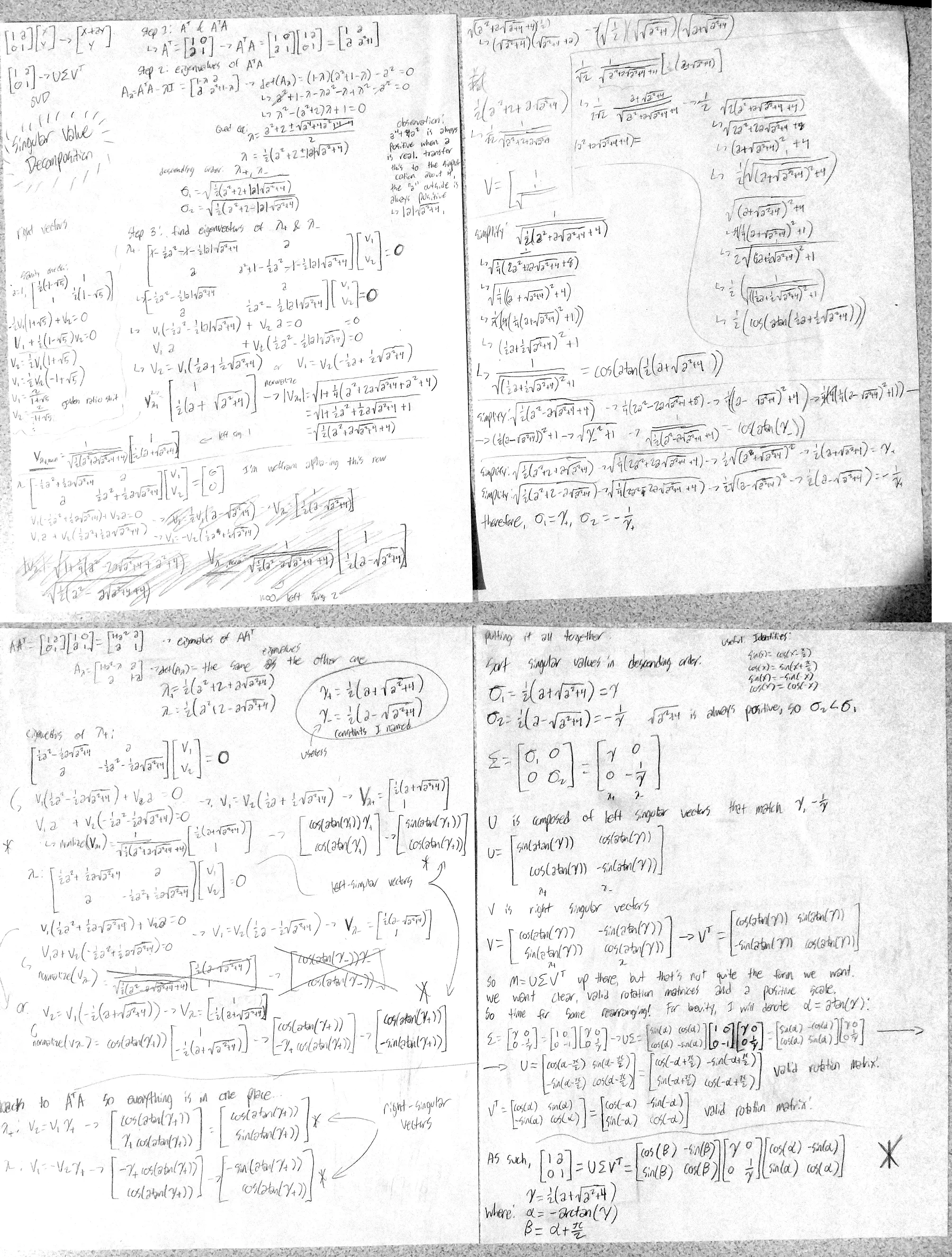
and, for completion’s sake, here’s the four main pages of work that I did for this problem:

four pages of dense math

further endeavors

I want to eventually derive the same equation for an arbitrary 3x3 “shear” matrix:

\begin{bmatrix}1&a&b\\ d&1&c\\ e&f&1\end{bmatrix}

but that will be for when I’m particularly bored one day, as I don’t envision it to be very fun, even when I can get wolfram alpha to do lots of the heavy lifting for me.

perhaps other funny matrix transformations can be derived in a similar way

back